Is gravity quantized? Entanglement witnesses aim to answer through the entanglement a gravitational interaction can create [1, 2]. Classical–quantum (CQ) gravity answers the other way: it keeps the metric classical and couples it to quantum matter by a linear, completely positive (CP) dynamics [3]. The price is fixed by positivity. A classical field that responds to quantum matter must diffuse, and the matter must decohere, with the product of the two bounded below: the decoherence–diffusion trade-off [4]. In the Newtonian limit the least decoherence allowed is the Diósi–Penrose rate [5, 6, 7], whose spontaneous X-ray emission is bounded by underground detectors [8, 9, 10].
A covariant version exists. Its diffusion kernel is quadratic in curvature, of DeWitt form \(\alpha R_{\mu\nu}R^{\mu\nu}-\beta R^2\) [11]; it is power-counting renormalisable with a positive scalar sector [12], and its scalar–vector–tensor decomposition shows a dynamical, stochastic conformal mode beside the spin-2 mode [13]. Its authors find it viable against matter-wave coherence, LISA Pathfinder and gravitational-wave data [13]. They find that with scale-independent couplings the integrated energy density of the stochastic gravitational waves would rule the theory out, and that asymptotic freedom [12] makes the coupling run [13]. The question of this paper is whether the covariant theory also survives the search for spontaneous X-rays.
Oppenheim and Panella expected anomalous heating bounds to be the most stringent [14], but did not compute them. They also noted that the tensor trade-off decoheres the strain components of the stress tensor, for example through \(T_{ij}T^{ij}\), so that it is unclear whether heating constrains the tensor coupling [14]. Diósi showed that the heating of Lorentz-invariant Markovian decoherence and diffusion diverges [15, 16]. The published X-ray bounds are for the Newtonian, frame-fixed model. An X-ray of energy \(E\) is emitted from noise at the frequency \(E/\hbar\). The assessment of the covariant theory rests on its static and low-frequency scalar sector and on its tensor sector at gravitational-wave frequencies [13]; the matter noise at keV frequencies was not evaluated.
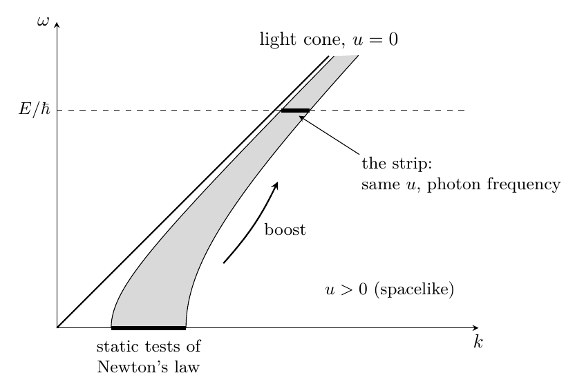
This paper computes the keV matter noise of covariant CQ gravity and confronts it with the XENONnT spectrum [10]. The idea fits in one line. Lorentz invariance maps the laboratory band on which Newton’s law is tested, invariant lengths from 1 mm to 1 m, onto a thin strip next to the light cone at every X-ray energy; the trade-off forces noise on that strip; slow matter feels it through its rest mass and radiates it as keV photons. The number is \[\begin{equation} \frac{\int s\,du}{\text{limit}}\;\geq\;\frac{\tfrac23\ln10^{6}}{7.7\times10^{-8}} \;=\;1.2\times10^{8}, \label{eq:headline} \end{equation}\] with \(s\) the matter noise in units of the Diósi–Penrose kernel and \(u=p^2\) the invariant momentum squared (Section 3). The limit is not a published number: it comes from our likelihood fit to the published spectrum (Section 5). After a bound-electron envelope we quote the exclusion as \(\geq1.1\times10^{8}\) for the observed spectrum; the median expected margin is \(6.6\times10^{7}\). The exclusion holds for every DeWitt coupling, every regulator and every running coupling that depends on \(p^2\) alone, and it needs Lorentz invariance of the scalar sector only up to boosts of about \(10^{7}\) (the margin is one at \(\gamma=1.1\times10^{7}\); this threshold is set by the 1–2.2 keV bins alone, and moves by about \(10\%\) between observed and median-expected data and between two evaluations of the atomic factor).
The scalar exclusion has a precise escape: a frame acting on the scalar sector. One of the authors’ completions, which puts a unit timelike vector into the scalar weight [13], survives it; so does a preferred foliation of the Hořava type [17, 18]. Section 6 answers that escape with a second argument, which rests on a further assumption and on an estimated margin. General relativity’s response to a conserved near-null source has a light-cone pole, and the pole is purely tensor. The response-squared form of the trade-off holds for every positive diffusion weight, so no frame in the weight removes it. It assumes general relativity’s tensor propagator at keV momenta, but it needs no transfer of static tests through Lorentz boosts. The atom’s Coulomb field gives the tensor source an order-one share. Its margin, \(1.7\times10^{9}\) (median expected \(9.8\times10^{8}\)), is an estimate, because the tensor conversion uses the elastic structure factor of an isolated atom. The two exclusions share several steps, which Section 6.5 lists; they are independent in the sense that different escapes defeat each. Section 2 gives both arguments in words and one picture, before any formalism.
The statements below are of three kinds, and the text says which is which. The two noise floors (Theorems 4.2 and 6.1) and the per-momentum trade-off they rest on (Lemma 3.1) are shown analytically from stated assumptions. The limit on the integrated noise and every margin are numerical: they come from a likelihood fit to the published spectrum with a model atom. The tensor margin, and the margin for a coupling that omits the Coulomb field, are estimates. Only the numbers that carry the result are in the body; Appendix A collects the rest.
We do not show that gravity is quantized. The scalar exclusion is conditional on a scalar sector that is Lorentz invariant up to boosts of about \(10^{7}\); with a frame in the scalar weight, or a non-perturbative scalar mass above \((0.34~\mu\mathrm{m})^{-1}\), it no longer applies. The tensor floor is shown for a tensor sector that is general relativity’s at keV momenta, where it has not been tested, and for matter coupled through its total stress, the Coulomb field included; its margin is an estimate, made with the elastic structure factor of an isolated atom, and no tensor conversion for liquid xenon with a relativistic atom is given. For a coupling that omits the Coulomb stress we have only a rough, gauge-dependent estimate. Whether the published theory is completely positive once matter is coupled is left open by its authors, and we do not settle it: the result is a dilemma between the theory as it stands and its completions (Section 7.2). The theorems are for Gaussian dynamics at linear order. For a Poisson record of jumps the floors and the mean photon yield are unchanged under stated conditions (Section 7.6), but a theory whose non-Gaussian noise delivers its keV emission in multi-photon bursts is not excluded, and jump dynamics outside those conditions are not treated. Nor do we exclude a theory with a non-linear effect that changes the scalar propagator next to the light cone and leaves the static sector alone. Frame-fixed Newtonian models are outside the result and remain subject to the published bounds [8, 10]. Sections 7 and 8 give the full scope.
The dynamical scalar is Oppenheim and Sajjad’s; its positivity is from [12]. So is the static scalar floor, a factor \(25/9\) above the tensor channel’s in their product of diffusion and decoherence; Remark 4.1(iii) gives its square root, \(5/3\), in our units [13]. That the tensor channel decoheres the transverse-traceless anisotropic stress is stated in [14] and [13]. The trade-off, and the remark that heating bounds on decoherence bound diffusion through it, are from [4]. The divergence of Lorentz-invariant Markovian heating is Diósi’s [15, 16]. The X-ray route was named in [14], and X-ray bounds on Newtonian CQ gravity follow from Tilloy and Diósi’s identification of its least-decoherence limit with the Diósi–Penrose model [6]. Gravitational-wave strain noise [19] and classical–quantum scattering [20] have been used against covariant CQ models by other routes. The conversion of noise into photons is Manti et al.’s [21]. What we add is the near-cone face of the conformal mode, the \(\alpha\)-independent floor that survives every \(p^2\)-only regulator, the tensor floor that survives every positive weight, the observation that an atom’s Coulomb field makes the tensor channel of order one at keV, the quantitative XENONnT bound on the scalar sector, and an estimate of the corresponding tensor margin. We found no earlier X-ray bound on covariant CQ gravity.
Section 2 states the idea. Section 3 sets up the Gaussian CQ dynamics and derives the trade-off at fixed momentum. Section 4 gives the scalar floor, Section 5 its conversion into photons and the XENONnT exclusion, Section 6 the tensor exclusion, Section 7 the objections and the scope, and Section 8 what remains. Appendix A lists the numerical values.
A classical field that carries a force between quantum bodies must be noisy, and the noise is at least as large as the response it carries. Where the response of gravity is known, the noise is therefore bounded below. Lorentz invariance, or the propagator of gravitational waves, places a known response next to the light cone at X-ray frequencies, and an atom turns noise there into photons that a detector counts.
The trade-off. A classical gravitational field that responds to quantum matter keeps a record of where the matter is. Positivity of the dynamics then demands two things at once: the record diffuses, and the matter decoheres, and the two cannot both be small. In one form, valid for any diffusion, the total noise that matter feels on a given source is at least the response of the mean field on that source (Eq. \(\eqref{eq:response-form}\)). At zero frequency this is the known statement that the least noise of a Newtonian classical field is the Diósi–Penrose kernel [6]. We measure every noise in units of that kernel and call it \(s\): the static Newtonian minimum is \(s=1/k^2\) at wavenumber \(k\).
The picture. Figure 1 shows the plane of frequency \(\omega\) and wavenumber \(k\) of the noise. Laboratory tests of Newton’s law are static: they sit on the axis \(\omega=0\), at \(k\) between \((1~\mathrm{m})^{-1}\) and \((1~\mathrm{mm})^{-1}\). A Lorentz-invariant kernel depends on \(\omega\) and \(k\) only through \(u=k^2-\omega^2\), so it is constant on each hyperbola of fixed \(u\), and each hyperbola runs from the static axis up along the light cone. An atom that emits a photon of energy \(E\) draws on the noise at the frequency \(\omega=E/\hbar\). On that line the tested band, \(u\) from \(1\) to \(10^{6}~\mathrm{m^{-2}}\), is a strip just outside the cone, at wavenumbers that exceed \(\omega/c\) by the relative amount \(u/2k^2\) to leading order. Noise on the strip has the wavelength of the photon, not of the laboratory. What Newton’s law fixes at a millimetre, Lorentz invariance repeats at every X-ray energy.
First argument: the scalar strip. The direct route fails, and the reason is instructive. In general relativity the Newtonian potential obeys a constraint, not a wave equation: its mean response to a conserved source has no pole on the light cone (Eq. \(\eqref{eq:shield}\)), so “noise at least as large as the response” gives slow matter nothing there. The covariant theory supplies the noise by another route. Its diffusion weight, with strength \(\alpha\), makes the conformal part of the metric a dynamical random field whose variance on the strip grows as \(1/(\alpha u^2)\). Positivity ties the direct decoherence of matter to the same weight, in proportion to \(\alpha\). Matter is therefore caught between two channels, one that grows and one that falls with \(\alpha\), and the sum is at least twice their geometric mean, in which \(\alpha\) cancels. The result is a floor, \(s\geq\tfrac23|f|/u\) (Theorem 4.2), with \(|f|=1\) wherever Newton’s law holds. It is two thirds of what a classical field coupled to the trace alone gives by the direct route. Integrated over the tested band it is \(\tfrac23\ln10^{6}=9.2\), the same at every X-ray energy.
An atom reads this noise because its matter and its field respond differently. Next to the cone the fluctuating metric is conformal. A slow particle feels a conformal mode through its rest mass and is accelerated; Maxwell’s equations are conformally invariant and do not see it. The charge is shaken relative to its own field and radiates. A neutral atom shaken as a whole radiates through the difference between its nuclear charge and its electronic form factor, which cancels only at long wavelength; from 10 to 140 keV the atomic factor lies between a quarter and one. Our likelihood fit to the spectrum of XENONnT’s search for such photons bounds the integrated noise at \(7.7\times10^{-8}\) in the same units, a factor of at least \(1.1\times10^{8}\) below the floor (median expected \(6.6\times10^{7}\)).
Within the Gaussian class at linear order, three things defeat this argument. The floor needs a diffusion weight that is built from Lorentz-invariant projectors; a preferred frame in the scalar weight breaks that structure, and the floor is then not shown: the one completion of this kind that the theory’s authors work out survives the scalar strip (Section 7.2). The transfer from the static axis to the strip needs Lorentz invariance of the scalar sector up to boosts of about \(10^{7}\). A scalar mass above \((0.34~\mu\mathrm{m})^{-1}\), which would have to be non-perturbative, lowers the floor below the limit. Regulators and running couplings that depend on \(p^2\) alone defeat nothing, because they are functions of \(u\) and the floor holds at each \(u\).
Second argument: the tensor strip. The pole that the Newtonian potential lacks is not absent from general relativity; it sits in the transverse-traceless part of the response, where gravitational waves propagate. On a transverse-traceless source next to the cone the response is \(2/u\), and here the direct route works: the noise is at least the response, \(s\geq2/u\) per polarisation, for every positive diffusion weight, with or without a frame (Theorem 6.1). Nothing is carried over from static tests. The input is that the mean tensor field of the theory is that of general relativity at keV momenta, which is an assumption: gravitational-wave observations test it only at far lower frequencies.
That an atom at rest should source a tensor mode is not obvious, since the stress of its moving particles is of order \(v^2/c^2\). The stress of its Coulomb field is not small. The field energy is part of the atom’s mass, the Maxwell stress is of the same order, and it is part of the conserved stress tensor, to which we assume the classical field couples. Tensor noise acting on the Coulomb field produces photons: at its floor, at no less than the rate of trace noise of strength \(X_{\rm TT}/u\), with a conversion ratio \(X_{\rm TT}\) that rises from \(1.6\) at 5 keV to \(9.6\) at 140 keV (Proposition 6.2). The resulting margin is \(1.7\times10^{9}\) (median expected \(9.8\times10^{8}\)). It is an estimate, not a bound: the conversion is computed for an isolated atom with its elastic structure factor.
Two things defeat the tensor argument and leave the scalar argument standing. One is a tensor sector whose pole has left the light cone at keV momenta, which for a Lifshitz dispersion with \(z=3\) requires a scale below about 10 eV. The other is a matter coupling that does not see the stress of the atom at all. A frame in the diffusion weight changes the inner product in which the bound is taken and leaves the bound in place. A frame placed elsewhere, in the matter coupling itself or as a cut-off below keV on the whole mean field, would defeat both arguments (Section 7.5).
What survives. A classical theory of the Gaussian class must defeat both arguments at once, or leave the class. For noise made of Poisson jumps the floors and the mean number of photons stay as they are under stated conditions, and leaving the class helps only if nearly all of the keV photons arrive in multi-photon bursts of a kind the detector’s event selection would reject (Section 7.6). The table of Section 6.5 sets the escapes side by side.
This section fixes the units, states the trade-off between decoherence and diffusion, and turns it from a statement about regions of spacetime into a statement at each momentum, the form in which both floors use it.
Signature \((-,+,+,+)\); \(c=1\) in formulas, SI in numbers. For a four-momentum \(p=(\omega,\mathbf{k})\), \[\begin{equation} u\equiv p^2=k^2-\omega^2 , \label{eq:u} \end{equation}\] so \(u>0\) is spacelike and the light cone is \(u=0\). Matter noise acts on the rest-mass density \(\rho_{m}=-T^{\mu}{}_{\mu}\) and enters a branch pair through the decoherence exponent \(-\tfrac12\int d^4p\,(2\pi)^{-4}|\Delta\rho_{m}(p)|^2S(p)\). Here \(\Delta\rho_{m}\) is the difference of the rest-mass density between the two branches and \(S(p)\) the noise kernel. We quote it in units of the Diósi–Penrose kernel, \[\begin{equation} s\equiv\frac{\hbar S}{4\pi G},\qquad s_{\rm DP}=\frac{1}{k^2}\ \text{at }C=1,\qquad s=\frac{N}{4\pi\lP^2},\quad 4\pi\lP^2=\frac{4\pi\hbar G}{c^3}=3.28\times10^{-69}~\mathrm{m^2}, \label{eq:s} \end{equation}\] with \(N\) (m\(^4\)) a kernel per unit \(\rho_{m}^2\), \(\lP\) the Planck length, and \(C\) the dimensionless strength that multiplies the Diósi–Penrose kernel. A detector bounds the noise as a whole, strength times kernel, so limits are written for \(C\int s\,du\); the floors below are lower bounds on the whole noise, written \(s\) with no separate strength. The Newton form factor \(f(u)\) is the classically carried response relative to Newton’s, \(|f|=1\) where Newton’s law is tested. A margin is the lower bound on \(\int s\,du\) divided by the upper limit on \(C\int s\,du\) that we obtain from the XENONnT spectrum (Section 5); a margin above one excludes.
In continuous (Gaussian) CQ dynamics [4, 11, 22] a classical record \(r\) couples to quantum matter branches \(m^\pm\) through three kernels: the decoherence kernel \(D_0\), the diffusion \(D_2\) of the record, and the drift \(D_1\) that carries the mean field. The weight on a branch pair is \[\begin{equation} W=\exp\Big\{-\tfrac12\Delta m\,D_0\,\Delta m -\tfrac12(r-D_1\bar m)\,D_2^{-1}(r-D_1\bar m) -\tfrac{i}{\hbar}\!\int\!\varphi\,\Delta m\Big\},\qquad \varphi=4\pi G\,\mathcal{G}_{\rm ret}*r . \label{eq:weight} \end{equation}\] Here \(\Delta m=m^+-m^-\) and \(\bar m\) are the difference and the mean of the two branches, \(\mathcal{G}_{\rm ret}\) is the retarded Green function, and \(\varphi\) is the potential that the record exerts on the matter. For a fixed record, \(W\) is a positive-definite kernel on path pairs on a region if and only if \[\begin{equation} K\equiv D_0-\tfrac14D_1^{\sf T}D_2^{-1}D_1\succeq0 \label{eq:tradeoff} \end{equation}\] on that region: the decoherence–diffusion trade-off [4, 11]. At \(\omega=0\) it states that a classical mediator’s noise is at least its full response, \(D\geq|\chi|/\hbar\) for decoherence kernel \(D\) and response \(\chi\), the static form of Tilloy and Diósi [6].
The trade-off \(\eqref{eq:tradeoff}\) is a statement about regions. The floors below need it momentum by momentum, and the passage is not automatic, because the inverse of a kernel restricted to a region is not the restriction of its inverse. The lemma shows that translation invariance, with positivity on every past region, closes the gap.
Lemma 3.1. Let \(D_0,D_1,D_2\) be translation invariant on Minkowski space, with locally integrable, polynomially bounded symbols on the physical record space, and let the dynamics be CP on every past region \(\Omega=\{t_i<t<t_f\}\), with kernels on \(\Omega\) the restrictions of the global ones. Then, for almost every \(p\), near-null \(p\) included, \[\begin{equation} \tilde D_0(p)\;\succeq\;\tfrac14\,\tilde D_1(p)^\dagger\,\tilde D_2(p)^{-1}\,\tilde D_1(p). \label{eq:tradeoff-p} \end{equation}\]
Proof. For \(A\succ0\), \(\langle w,A^{-1}w\rangle=\sup_\psi\,[2\langle w,\psi\rangle-\langle\psi,A\psi\rangle]\). CP on \(\Omega\) therefore gives \(\langle f,D_0f\rangle\geq\tfrac14(2\langle D_1f,\psi\rangle-\langle\psi,D_2\psi\rangle)\) for every \(\psi\in C_c^\infty(\Omega)\) and every \(f\) supported in \(\Omega\); only \(D_1f\) on \(\operatorname{supp}\psi\) enters. For fixed \(f\), translation invariance lets \(\Omega\) be shifted and enlarged to contain any compact set, so the inequality holds for every \(\psi\in C_c^\infty(\mathbb{R}^4)\). \(C_c^\infty\) is dense in the form domain of a tempered, locally integrable symbol and Plancherel holds in any signature, so the supremum is \(\tfrac14\int|\tilde D_1\tilde f|^2/\tilde D_2\,d^4p/(2\pi)^4\). Wave packets concentrated at \(p\) give \(\eqref{eq:tradeoff-p}\). ◻
The lemma means that the decoherence of matter at one four-momentum is bounded below by the drift and the diffusion at the same four-momentum, with no reference to a region. Both floors below are evaluations of \(\eqref{eq:tradeoff-p}\) at momenta next to the light cone.
Remark 3.1. On any fixed region the compressed kernel satisfies \((D_2|_\Omega)^{-1}\prec(D_2^{-1})|_\Omega\), and near the cone the gap is large; CP on one region does not imply \(\eqref{eq:tradeoff-p}\). For translation-invariant kernels, CP on every past region does. A packet at the lower edge of the band, \(u=1~\mathrm{m^{-2}}\), on the 140 keV shell needs a null extent \(k/u\) that is far below the Hubble length (Appendix A), so the finite age of the universe does not reopen the gap. A kernel that is CP region by region but not translation invariant carries an origin or a frame; it belongs to the shielded class of Section 7.
The same steps at one momentum give a second form of the trade-off, which bounds the noise by the response of the mean field and does not refer to the diffusion weight. With \(S(J)=\langle J,D_0J\rangle+c_G^2\langle\mathcal{G}J,D_2\mathcal{G}J\rangle\) the total noise on a source \(J\), \(c_G=4\pi G/\hbar\) and \(\mathcal{G}\) the propagator of the mean field, Cauchy–Schwarz in the \(D_2\) inner product and the arithmetic–geometric mean inequality give \[\begin{equation} S(J)\;\geq\;c_G\,\big|\langle D_1J,\mathcal{G}J\rangle\big| , \label{eq:response-form} \end{equation}\] whatever the form of \(D_2\). In units \(\eqref{eq:s}\) this reads \(s\geq|f|/u\) for a scalar source with a retarded drift (retarded and advanced agree at spacelike \(p\)). For a drift that depends on \(u\) alone, static Newton fixes \(|f(u)|=1\) on \(u\in[1,10^{6}]~\mathrm{m^{-2}}\). The tensor floor of Section 6 is \(\eqref{eq:response-form}\) on a transverse-traceless source. The scalar floor of Section 4 cannot use it, for a reason given there, and uses \(\eqref{eq:tradeoff-p}\) with the form of the diffusion weight.
The covariant diffusion makes the conformal part of the metric a random field with large variance next to the light cone. This section shows that slow matter feels that field through its rest mass, that the mean field gives no bound there, and that the two noise channels of the theory together give a floor that does not depend on the couplings.
Linearised about Minkowski space, covariant CQ gravity gives the metric perturbation \(h\) the weight [11, 12, 13] \[\begin{equation} \exp\Big\{-\tfrac12\!\int\!\big(\alpha R_{\mu\nu}R^{\mu\nu}-\beta R^2\big)\Big\},\qquad b\equiv\beta/\alpha<\tfrac13 , \label{eq:dewitt} \end{equation}\] a diffusion with DeWitt form \(D_2^{-1}=\alpha I-\beta\eta\eta\), where \(R_{\mu\nu}\) and \(R\) are the linearised Ricci tensor and scalar of \(h\), \(\eta\) is the Minkowski metric, and \(\alpha\), \(\beta\) are the two couplings of the theory. The explicit decoherence term is \(\tfrac18\Delta T\,D_0\,\Delta T\) with \(D_0\succeq64\pi^2G^2D_2^{-1}\), saturated by the authors. Matter couples through \(\tfrac12h_{\mu\nu}T^{\mu\nu}\). In the scalar–vector–tensor split the conformal scalar \(\psi\) and the transverse-traceless part \(h^{\mathrm{TT}}\) are dynamical, and the Bardeen potential \(\Phi\), which is the potential that accelerates slow matter, and the vector \(V_i\) are constraints [13]. The scalar correlator is [13] \[\begin{equation} \langle\Phi\Phi\rangle=\frac{3}{2\alpha k^4} +\frac{1}{\alpha p^4}\Big[\frac{\omega^2}{k^2}+\frac{-3\alpha+10\beta}{4(\alpha-3\beta)}\Big]. \label{eq:phiphi} \end{equation}\] We rederived \(\eqref{eq:phiphi}\) from the quadratic form of \(\eqref{eq:dewitt}\), with the four gauge modes removed and the Bardeen functionals \(\Phi=\tfrac12h_{00}+\tfrac{\omega}{k}\hat k\cdot h_0+\tfrac{3\omega^2}{4k^2}(\hat k\hat k-\tfrac13\delta){:}h\), \(\psi=\tfrac14(\delta-\hat k\hat k){:}h\).
The proposition evaluates this correlator next to the cone. It shows that the variance of \(\Phi\) has a double pole in \(u\) there, and that the fluctuation is conformal: \(\Phi+\psi\), which measures the departure from a conformal metric, stays small.
Proposition 4.1. On the strip \(u\ll k^2\), \[\begin{equation} \langle\Phi\Phi\rangle=\frac{c_d(b)}{\alpha u^2}-\frac{1}{\alpha k^2u}+O(1),\qquad c_d(b)=\frac{1-2b}{4(1-3b)}, \label{eq:cd} \end{equation}\] with \(c_d\in[\tfrac16,\tfrac12]\) for \(b\leq\tfrac14\). At every \(p\), \(\langle(\Phi+\psi)^2\rangle=3/(2\alpha k^4)\), so that \[\begin{equation} \frac{\langle(\Phi+\psi)^2\rangle}{\langle\Phi^2\rangle}=\frac{3}{2c_d}\Big(\frac{u}{k^2}\Big)^2\big[1+O(u/k^2)\big] \leq9\Big(\frac{u}{k^2}\Big)^2\big[1+O(u/k^2)\big]. \label{eq:conformal} \end{equation}\] Near the cone \(h_{\mu\nu}\approx2\psi\eta_{\mu\nu}\): a conformal mode.
Proof. At \(p^4=u^2\) and \(\omega^2/k^2=1-u/k^2\) the bracket of \(\eqref{eq:phiphi}\) is \(1+\frac{-3+10b}{4(1-3b)}-\frac{u}{k^2}=\frac{1-2b}{4(1-3b)}-\frac{u}{k^2}\), which gives \(\eqref{eq:cd}\). For \(\Phi+\psi\): on \(h=2\sigma\eta\) the functionals give \(\Phi=-\sigma\), \(\psi=\sigma\), so \(\Phi+\psi\) is gauge and Weyl invariant. At quadratic order \(R_{\mu\nu}R^{\mu\nu}=\tfrac12C_{\mu\nu\rho\sigma}C^{\mu\nu\rho\sigma}+\tfrac13R^2\) up to a total derivative, with \(C_{\mu\nu\rho\sigma}\) the linearised Weyl tensor and \(C^2\) its square, so the weight is \(\tfrac\alpha2C^2+\alpha(\tfrac13-b)R^2\) with both coefficients positive for \(b<\tfrac13\). On the scalar sector, where \(\Phi+\psi\) lives and the weight is positive, the variance of a linear functional \(L\) is \(\sup_h(Lh)^2/(\text{weight})\); over all \(h\) the supremum would be infinite, since the vector weight is negative at spacelike \(p\) (Section 7.2). Since \(R(2\sigma\eta)\propto p^2\sigma\neq0\) off the cone, every \(h\) can be shifted along the conformal direction to \(R=0\) without changing \(L=\Phi+\psi\) or \(C_{\mu\nu\rho\sigma}\); the supremum is therefore attained at \(R=0\), and it does not depend on \(b\). Evaluating the quadratic form gives \(3/(2\alpha k^4)\); the value was also checked numerically across the range of \(b\) and \(\omega/k\) (Appendix A). Dividing by \(\eqref{eq:cd}\) and using \(c_d\geq\tfrac16\) for every \(b<\tfrac13\) gives \(\eqref{eq:conformal}\). ◻
The proposition means that on the strip the potential that accelerates slow matter fluctuates with a variance \(c_d/(\alpha u^2)\), larger the weaker the diffusion weight \(\alpha\), and that this fluctuation is a rescaling of the metric. Only the lower bound \(c_d\geq\tfrac16\) is used below, and it holds for every \(b<\tfrac13\); the upper bound \(\tfrac12\) holds for \(b\leq\tfrac14\), where the DeWitt form \(\alpha I-\beta\eta\eta\) is non-negative on every component of \(h\) and not only on the physical modes. The next subsection shows why such a rescaling shakes charges without shaking their fields.
On a conserved near-null source (Section 4.4) \[\begin{equation} \tfrac12h_{\mu\nu}J^{\mu\nu}=(\Phi+\psi)\rho-\psi\rho_{m}\;\approx\;\Phi\,\rho_{m}, \label{eq:coupling} \end{equation}\] so the mode couples to the rest-mass density \(\rho_{m}=-T^\mu{}_\mu\); the traceless electromagnetic binding fields drop out. A slow particle has geodesic acceleration \(\mathbf a=+\nabla\Phi\) (with \(\Phi=\tfrac12h_{00}+\dots\) a static mass \(M\) at distance \(r\) has \(\Phi=+GM/r\)). Maxwell’s equations are conformally invariant in four dimensions, so the photon field does not see the mode: in conformal variables Maxwell is flat and the rest mass varies, a slow charge has coordinate acceleration \(+\nabla\Phi\) and radiates by Larmor, with no Coulomb-scattering term to cancel it. The non-conformal remainder is \(O(u/k^2)\), which is negligible on the band at X-ray energies (Appendix A). Near the cone the scalar sector of covariant CQ gravity acts on slow matter as a stochastic Nordström field.
The response form \(\eqref{eq:response-form}\) bounds noise by the response of the mean field, so the first question is what that response is next to the cone. General relativity’s retarded response of \(\Phi\) to any conserved source, with energy density \(\rho\), stress \(\tau_{ij}\) and transverse stress trace \(\operatorname{tr}_\perp\tau\equiv(\delta_{ij}-\hat k_i\hat k_j)\tau_{ij}\) (the \(\operatorname{tr}\Sigma\) of Eq. \(\eqref{eq:source}\) below), is \[\begin{equation} \frac{\Phi_{\rm resp}}{16\pi G}=\frac{1}{k^2}\Big[-\frac{\rho-\operatorname{tr}_\perp\tau}{4}+\frac{\rho u}{2k^2}\Big], \label{eq:shield} \end{equation}\] with no pole at \(u=0\): the instantaneous Poisson constraint at every \(\omega\). The \(1/u\) response sits in the tensor channel (Section 6). The response form \(\eqref{eq:response-form}\) therefore gives slow matter no near-cone floor. The floor comes from the diffusion structure \(\eqref{eq:dewitt}\), through both channels at once.
The floor is a statement about the noise on the source that an emitting atom presents. Conservation fixes the form of that source next to the cone and shows which of its parts can carry a floor. At near-null \(p\) every conserved source has the form \[\begin{equation} J=A\,ll+B\,(le+el)+\Sigma_{ab}\,e_ae_b,\qquad l=\big(1,\tfrac{\omega}{k}\hat k\big),\quad l\cdot l=-\frac{u}{k^2},\quad e_a\perp\hat k , \label{eq:source} \end{equation}\] and conservation forces \(T^{0z}\approx T^{00}\). For a slow atom the relevant source is the transition element \(\langle f\gamma|T^{\mu\nu}(p)|0\rangle\) of the full emission process. It includes the photon and the Maxwell stress of the atom’s Coulomb field and is conserved because the total \(T^{\mu\nu}\) is, so \(\eqref{eq:source}\) is a property of the amplitude, not of the kinetic stress of the atom. The trace \(T\) of the source sits in the transverse block, \(\operatorname{tr}\Sigma=T+Au/k^2\approx-\rho_{m}\). Write \(\kappa\equiv\Sigma{:}\Sigma/\rho_{m}^2\geq\tfrac12\), with equality when the traceless part \(\Sigma^{\mathrm{TT}}\) vanishes. The saturated explicit kernel per \(\alpha\) splits as \[\begin{equation} \frac{N}{\alpha}=J{:}J-bT^2=\big(\tfrac12-b\big)(\operatorname{tr}\Sigma)^2+\Sigma^{\mathrm{TT}}{:}\Sigma^{\mathrm{TT}} -2B^2\frac{u}{k^2}+(1-b)A^2\frac{u^2}{k^4}+2bA\operatorname{tr}\Sigma\,\frac{u}{k^2}. \label{eq:split} \end{equation}\] The \(ll\) part, which carries \(T^{00}\), \(T^{0z}\) and \(T^{zz}\) together, has weight \((1-b)u^2/k^4\), which is negligible on the band at every energy above 1 keV (Appendix A): the energy density carries none of the floor. The trace enters with weight \(\tfrac12-b>0\), the anisotropic stress with weight one, and the \(B\) term, the non-positive direction of the DeWitt form, at \(O(u/k^2)\).
Matter on the source \(\eqref{eq:source}\) receives noise through two channels. The explicit channel is the decoherence that positivity ties to the diffusion weight; it is proportional to \(\alpha\). The dynamical channel is the fluctuating potential of Proposition 4.1; it is proportional to \(1/\alpha\). The theorem shows that their sum has a lower bound in which \(\alpha\) does not appear, and that the bound holds for every positive weight built from the two Lorentz-invariant projectors that act on conserved sources, the spin-2 projector \(P^{(2)}\) and the spin-0 projector \(P^{(0s)}\), with coefficients that are any positive functions of \(p^2\).
Theorem 4.2. Let the CQ dynamics be Gaussian, translation invariant and CP on every past region, with matter coupled through \(\tfrac12h_{\mu\nu}T^{\mu\nu}\) and Newton’s force carried by the classical field. Let the diffusion weight on physical modes be \(D_2^{-1}=a_2(p^2)P^{(2)}+a_0(p^2)P^{(0s)}\) with \(a_2,a_0>0\), the DeWitt form \(\eqref{eq:dewitt}\) included. Then on the conserved near-null source \(\eqref{eq:source}\) \[\begin{equation} s(u)\;\geq\;\frac23\,\frac{|f(u)|}{u}\,\big[1+O(u/k^2)\big] \label{eq:floor} \end{equation}\] for every \(\alpha\), every \(b<\tfrac13\) and every \(p^2\)-dependent regulator or running of \(a_2,a_0\).
Proof. For the DeWitt weight the two channels on the same source are \[\begin{equation} s_{\rm exp}=4\pi\lP^2\,\alpha(\kappa-b)\,|f|^2,\qquad s_{\rm dyn}=\frac{\kappa-\frac{1-4b}{4(1-3b)}}{4\pi\lP^2\,\alpha\,u^2}, \label{eq:channels} \end{equation}\] the first from \(\eqref{eq:split}\) with \(D_0\) saturating \(\eqref{eq:tradeoff-p}\) (Lemma 3.1), the second from \(\eqref{eq:cd}\) on the source. Both increase with \(\kappa\), so their product is least at \(\kappa=\tfrac12\): \[\begin{equation} s_{\rm exp}\,s_{\rm dyn}\geq\big(\tfrac12-b\big)c_d\,\frac{|f|^2}{u^2} =\frac{\tilde g^2|f|^2}{4u^2},\qquad \tilde g^2=\frac{(1-2b)^2}{2(1-3b)}\geq\frac49 , \label{eq:product} \end{equation}\] with the minimum at \(b=\tfrac16\). The product does not contain \(\alpha\), and \(s\geq2\sqrt{s_{\rm exp}s_{\rm dyn}}=\tilde g|f|/u\geq\tfrac23|f|/u\). For general positive \((a_2,a_0)\) the invariant form on conserved sources is \(\tfrac14J\langle hh\rangle J=(x_2/a_2+x_0/4a_0)/p^4\) with \(x_2=J\cdot P^{(2)}\cdot J\) and \(x_0=T^2/3\), and Cauchy–Schwarz gives \[\begin{equation} (a_2x_2+a_0x_0)\Big(\frac{x_2}{a_2}+\frac{x_0}{4a_0}\Big)\geq\big(x_2+\tfrac12x_0\big)^2\geq\frac{\rho_{m}^4}{9}, \label{eq:cs} \end{equation}\] since at \(\kappa\geq\tfrac12\), \(x_0=\rho_{m}^2/3\) and \(x_2\geq\rho_{m}^2/6\). The DeWitt weight at \(b=\tfrac16\) attains the bound. ◻
The theorem means that no choice of the couplings, and no regulator or running that is a function of \(p^2\), lowers the noise on the strip below two thirds of the value \(|f|/u\) that a field coupled to the trace alone would have: weakening one channel strengthens the other. The floor is analytic. Its assumptions are those of the statement; the one that a classical theory can give up at least cost is the form of the weight.
Remark 4.1. (i) The floor \(\eqref{eq:floor}\) is not the square of a response: the scalar response is shielded \(\eqref{eq:shield}\). It needs a weight diagonal in the Lorentz-invariant projectors. A frame in the scalar weight breaks this structure; Section 7.5 lists what that costs. (ii) At \(b\to\tfrac13^-\) the factor \(\tilde g^2\) rises monotonically from its minimum and diverges; at \(b=\tfrac13\) the scalar is Weyl-degenerate and unweighted, and \(b>\tfrac13\) is not positive. Nothing opens at the edge. Hirotani and Matsumura report that a strain-noise term vanishes at \(\beta=\tfrac13\) [19]; that factor comes from a non-conserved stochastic source in harmonic gauge, and on the conserved source \(\eqref{eq:source}\) the physical scalar weight is \(a_0=\alpha-3\beta\). (iii) At \(\omega=0\) conservation gives \(\kappa=1\) and the floor is \(\sqrt{(1-b)(3-8b)/(1-3b)}/k^2\geq\tfrac53/k^2\), above the static mediator value \(1/k^2\). This static floor is Oppenheim and Sajjad’s [13]. With \(x=1-3b\), \((1-b)(3-8b)/(1-3b)=(1+8x)(2+x)/(9x)\) is their ratio of the scalar channel’s product of diffusion and decoherence to the tensor channel’s, whose minimum \(25/9\) at \(b=\tfrac16\) they give. The noise floor is its square root, because the least noise is twice the geometric mean of the two channels.
The emission of an atom depends on the floor through its integral over the strip (Section 5), and static tests fix the integrand. Newton’s law is tested with \(|f|=1\) from 1 mm to 1 m, that is \(u\in[1,10^6]~\mathrm{m^{-2}}\). By Lorentz invariance of the scalar weights this band is a near-cone strip at every photon energy, and \[\begin{equation} \int s\,du\;\geq\;\frac23\ln10^{6}=9.21 . \label{eq:int-floor} \end{equation}\] For a theory whose classical field couples to the trace alone (Nordström-type CQ gravity [23]) the response form \(\eqref{eq:response-form}\) applies directly, \(s\geq|f|/u\), and \(\int s\,du\geq\ln10^6=13.8\). Both integrals depend on the tested band only through the logarithm of its width, and neither depends on the photon energy.
Noise on the mass density accelerates charges, and accelerated charges radiate. This section converts the floor into a photon spectrum, fits it to the XENONnT data, and finds how much Lorentz invariance the exclusion uses. The floor is analytic; the conversion uses a model atom and the limit is a numerical fit, so every margin in this section is numerical.
For Gaussian noise on the mass density with \(\langle\varphi\varphi\rangle(\mathbf q)=\hbar^2D(\mathbf q)\), every particle receives the mass-independent acceleration \(-\nabla\varphi\). Closure over atomic final states gives the photon spectrum per atom \[\begin{equation} \frac{d\Gamma}{dE}=\frac{e^2\hbar}{4\pi^2\varepsilon_0c^3E}\int\!\frac{d^3q}{(2\pi)^3}\, D(\mathbf q)\,q^2\,\big\langle\sin^2\!\angle(\mathbf q,\mathbf k)\;S(|\mathbf q-\mathbf k|)\big\rangle_{\hat k}, \qquad k=\frac{E}{\hbar c}, \label{eq:rate} \end{equation}\] with \(D(\mathbf q)\) the noise kernel at frequency \(E/\hbar\), \(\mathbf k\) the photon wavevector, and \(S(Q)=|Z-F(Q)|^2+\sum_an_a(1-f_a^2)\) the charge structure factor of the atom of nuclear charge \(Z\): \(F\) is the electronic form factor, and \(n_a\), \(f_a\) are the occupation and form factor of orbital \(a\). The first term is elastic (the atom stays in its ground state), the second inelastic, in the product-density approximation. This is Manti et al.’s rate for a stationary correlation [21] evaluated on the near-cone correlation; for smooth noise it reduces to the Diósi–Penrose pair formula of XENONnT [10]; that of Donadi et al. [8] has the same form with a coefficient larger by \(8\pi\). A shaken neutral atom radiates through \(Z-F(Q)\), which vanishes only as \(Q\to0\): the atomic cancellation is strong only at the lowest energies of the window, where the wavelength exceeds the size of the atom (\(A_{\rm cone}=0.002\) at 1 keV), and is weak at the energies that set the limit.
Near-cone noise has \(|\mathbf q|=k\) and is isotropic, so the structure factor is sampled at the Thomson momentum transfer \(Q=2k\sin(\theta/2)\). Relative to the uncorrelated value \(Z^2+Z\), \[\begin{equation} A_{\rm cone}(E)=\frac{\big\langle\tfrac32\sin^2\theta\;S(2k\sin\tfrac\theta2)\big\rangle}{Z^2+Z}, \label{eq:acone} \end{equation}\] the average being over the angle \(\theta\) between noise and photon. In the closure approximation this atomic factor is the whole effect of atomic structure on the signal. For an isolated xenon atom in the local-density approximation it rises from \(0.258\) at 10 keV to \(0.955\) at 140 keV (Table 5): at the energies that set the limit, 50–140 keV, it is \(0.79\) or more. The emission integral \(I(E)=2\pi\int(u+E^2)^{3/2}s\,du\geq2\pi E^3\int s\,du\) makes the \(E^2A_{\rm cone}\) template a lower bound on the signal, so the data constrain the integrated noise \(\int s\,du\).
The rate \(\eqref{eq:rate}\) is for noise that accelerates every particle, as the conformal mode does. Part of the floor is of another kind: the explicit channel is decoherence of a stress component, not a fluctuating potential. This subsection shows that it radiates with the same atomic factor, so that the floor can be used as a whole. The floor of Theorem 4.2 sits on the explicit channel’s coupling to \(\operatorname{tr}\Sigma=-\rho_{m}\). Noise on that trace is the transverse-trace metric \(h_{ab}=h_\perp\delta_{ab}\) (\(a,b\perp\hat q\)), whose Bardeen potentials are \[\begin{equation} \Phi=-\frac{h_\perp\omega^2}{2q^2},\qquad\psi=\frac{h_\perp}{2},\qquad\Phi+\psi=\frac{h_\perp u}{2q^2}, \label{eq:trace-mode} \end{equation}\] the conformal mode near the cone. For a metric mode acting on charges at rest with charge form factor \(R(Q)\), linearised geodesics and the linearised constitutive relations of the Coulomb field give a radiated field \(\propto\hat k\times\mathbf J\) with \[\begin{equation} \mathbf J=R(Q)\Big[\mathbf v+\omega\,\frac{\Delta\varepsilon\cdot\mathbf Q}{Q^2} -\frac{\mathbf k\times(\mathbf g\times\mathbf Q)}{Q^2}\Big],\qquad \Delta\varepsilon_{ij}=\big(\tfrac12h_{00}+\tfrac12\operatorname{tr}h\big)\delta_{ij}-h_{ij},\quad g_i=h_{0i}, \label{eq:amplitude} \end{equation}\] \(\mathbf v\) the geodesic velocity. The last two terms are the Maxwell stress of the atom’s own Coulomb field. \(\mathbf J\) is invariant under \(h\to h+i(p\zeta+\zeta p)\) for any \(\zeta\) and off-shell \(\mathbf q\). For the trace mode \(\eqref{eq:trace-mode}\) it equals the Larmor amplitude of the conformal kick up to a relative remainder \(\leq3u/Q^2\). In the gauge where the noise couples only to stresses, the photon comes from the Coulomb field’s Maxwell stress, which is of order one, not from the particles’ kinetic stress, which is of order \(v^2/c^2\). Because the Maxwell stress tensor is traceless, the trace the floor uses is the rest-mass trace whether or not the noise couples to the Coulomb field. The floor and the field noise share one conversion, \(A_{\rm cone}\).
The limit is numerical. We fit the template \(E^2A_{\rm cone}\) to the XENONnT spectrum from 1 to 140 keV [10] with a profile likelihood, at one-sided 95% confidence; Appendix A gives the ingredients of the fit and its comparison with the published Diósi–Penrose limit, which it reproduces to within half a percent in that model’s smearing length, on the conservative side. With \(A_{\rm cone}\) interpolated through the five tabulated points, \[\begin{equation} C\int s\,du\;<\;7.7\times10^{-8}\qquad(\text{without the atomic factor: }7.4\times10^{-8}). \label{eq:limit} \end{equation}\] The atomic factor moves the limit by a few percent only, because the \(E^2\) template is dominated by 50–140 keV, where \(A_{\rm cone}\) lies between \(0.79\) and \(0.96\). The limit \(\eqref{eq:limit}\) is the one obtained from the observed spectrum; the median expected limit for a background-only spectrum is \(1.39\times10^{-7}\). The five-point interpolation underestimates the directly computed \(A_{\rm cone}\) by up to about \(40\%\) between 1 and 10 keV, which is conservative: with the computed factor the margin of row 1 of Table 1 moves from \(1.192\times10^{8}\) to \(1.198\times10^{8}\), and the boost threshold of Section 5.5 from \(1.06\times10^{7}\) to \(1.02\times10^{7}\).
| Row, applies to | \(\int s\,du\geq\) | Margin | |
|---|---|---|---|
| 1 | Floor \(\eqref{eq:floor}\) on \(u\in[1,10^6]~\mathrm{m^{-2}}\): every \(\alpha\), \(b<\tfrac13\), every invariant \((a_2,a_0)\) | 9.21 | \(1.19\times10^{8}\) |
| 2 | Field noise alone, constant couplings at the coherence edge \(D_{2,\rm scalar}\geq10^{-71}\) | \(1.9\times10^{-4}\) | \(2.5\times10^{3}\) |
| 3 | Invariant \(\varepsilon\) prescription, \(\langle\Phi\Phi\rangle=D_G/(p^4+\varepsilon^2)\), \(D_G\geq10^{-71}\) | \(3.05\times10^{-3}\) | \(3.9\times10^{4}\) |
| 4 | Trace-coupled (Nordström-type) CQ, \(s\geq|f|/u\) | 13.8 | \(1.79\times10^{8}\) |
Table 1 collects the margins. Row 1 is the result: the floor \(\eqref{eq:int-floor}\), which no coupling and no invariant regulator can lower, exceeds the limit by eight orders of magnitude. The other rows are cross-checks that drop one input each. Row 2 drops the trade-off: it integrates the field noise \(c_d/(\alpha u^2)\) alone from \(u=1~\mathrm{m^{-2}}\), \(\int s\,du=(c_d/\alpha)/(4\pi\lP^2\cdot1~\mathrm{m^{-2}})\), with constant couplings. At fixed scalar diffusion constant \(D_{2,\rm scalar}=(3\alpha-8\beta)/(\alpha(\alpha-3\beta))\), bounded below by matter-wave coherence [13, 14], \(\min_b(c_d/\alpha)/D_{2,\rm scalar}=\tfrac1{16}\), reached as \(b\to-\infty\); at \(b=0\) the margin is larger. For constant couplings, even where the diffusion is as weak as coherence allows, the fluctuating potential alone is excluded, by about \(2.5\times10^{3}\). Row 3 is the regulated form of [12] at the same coherence edge. Its normalisation is ambiguous by a factor of about four: with \(D_G\geq10^{-71}\) at face value the margin is \(3.9\times10^{4}\); if the edge is read on \(D_{2,\rm scalar}\) as in row 2, then \(D_G\geq2.5\times10^{-72}\), \(\int s\,du\geq7.6\times10^{-4}\) and the margin is \(9.9\times10^{3}\). The row excludes by about \(10^{4}\) to \(4\times10^{4}\). Row 4 is the response form \(\eqref{eq:response-form}\) for a scalar source.
The margin of row 1 depends on the atomic input at the level of ten percent. An envelope for the order-\(v^2/c^2\) correction of bound electrons to the coherent amplitude, \(c_v\in[-3,3]\) times the kinetic form factor, spans \(1.11\)–\(1.27\times10^{8}\) (Appendix A gives the other variants). We quote row 1 as \(\geq1.1\times10^{8}\). These are margins for the observed spectrum, whose limit is stronger than the median expected one; the median expected margin of row 1 is \(6.6\times10^{7}\).
The strip is the image of the laboratory band under a boost, and Lorentz invariance has not been tested at arbitrary boosts. The question is how large a boost the exclusion uses. The full margins use the strip up to 140 keV, which maps \(u=1~\mathrm{m^{-2}}\) onto the photon shell with a boost \(k/\sqrt u=7.1\times10^{11}\). Exclusion needs far less, because the margin is large and the upper part of the band needs smaller boosts. If the scalar sector is Lorentz invariant only up to \(\gamma_{\max}\), the usable strip at energy \(E\) is \(u\geq(k/\gamma_{\max})^2\). Refitting with the strip cut in this way (Table 6), the floor margin reaches one at \(\gamma_{\max}=1.1\times10^{7}\); the constant-coupling window (row 2) at \(\gamma_{\max}=1.6\times10^{10}\). These are the boosts at which the margins are exactly one; at \(\gamma_{\max}=1.2\times10^{7}\) the floor margin is \(2.1\). The threshold of the floor is set by the 1–2.2 keV bins alone: at \(\gamma_{\max}=1.1\times10^{7}\) the usable strip is empty above \(2.17\) keV. There the atomic factor is least accurate, so the threshold is approximate; between the interpolated and the directly computed atomic factor it is \(1.02\)–\(1.06\times10^{7}\) for the observed spectrum and \(1.13\)–\(1.19\times10^{7}\) for the median expected one, a spread of about \(10\%\). The scalar exclusion therefore needs a scalar sector that is Lorentz invariant up to boosts of about \(10^{7}\), and says nothing about a theory in which invariance fails below that.
The scalar floor needs a diffusion weight that is diagonal in the Lorentz-invariant projectors, and it needs Lorentz invariance to carry Newton’s tested band to the light cone. A frame in the scalar weight removes it (Section 7.5). This section shows that the tensor sector gives a noise floor that uses neither step, and estimates the exclusion that follows from it. The floor is analytic under three stated assumptions. The margin is an estimate, for the reasons collected in Remark 6.2, and is labelled so wherever it is quoted.
The scalar response has no pole on the light cone. The full response of general relativity has one, and conservation decides which part of the source carries it. Normalised so that a static density gives Newton’s response, \(\chi=\rho^2/k^2\), the response of general relativity to a conserved source \(J\) with trace \(T\) is \[\begin{equation} \chi(J)=\frac{2\,(J{:}J-\tfrac12T^2)}{u}. \label{eq:gr-response} \end{equation}\] On the near-null source \(\eqref{eq:source}\), the split \(\eqref{eq:split}\) at \(b=\tfrac12\) gives \[\begin{equation} J{:}J-\tfrac12T^2=\Sigma^{\mathrm{TT}}{:}\Sigma^{\mathrm{TT}}-2B^2\frac{u}{k^2}+\frac12A^2\frac{u^2}{k^4}+A\operatorname{tr}\Sigma\,\frac{u}{k^2}, \qquad \chi(J)=\frac{2\,\Sigma^{\mathrm{TT}}{:}\Sigma^{\mathrm{TT}}}{u}+O\big(k^{-2}\big). \label{eq:tt-response} \end{equation}\] The light-cone pole that the scalar response lacks \(\eqref{eq:shield}\) is entirely in the transverse-traceless block. It is the propagator of the theory’s own mean field: in the covariant theory the classical Einstein equation; in a theory with a preferred foliation, \(1/(c_T^2k^2-\omega^2)\) with a tensor speed \(c_T\) that obeys \(|c_T-1|\lesssim10^{-15}\) [24]. For \(c_T\neq1\) the strip is taken on the spacelike side of the tensor cone, where the response is real; the near-null relations \(\eqref{eq:source}\) then change at relative order \(|c_T-1|\), which we neglect.
Because the tensor response has a pole, the response form \(\eqref{eq:response-form}\) of the trade-off applies to it directly. The theorem shows that the noise on each transverse-traceless polarisation is then at least \(2/u\), and that the form of the diffusion weight does not enter.
Theorem 6.1. Assume
Gaussian CQ dynamics, translation invariant and CP on every past region;
a drift whose response on conserved sources at the near-null momentum \(p\) is the tensor response \(\eqref{eq:tt-response}\);
matter coupled through \(\tfrac12h_{\mu\nu}T^{\mu\nu}\) to the total conserved \(T^{\mu\nu}\), the atom’s Coulomb field included.
Then for every positive diffusion kernel \(D_2\), Lorentz invariant or carrying any frame, the matter noise on every unit transverse-traceless polarisation \(e\) obeys, in units \(\eqref{eq:s}\), \[\begin{equation} s_e(u)\;\geq\;\frac{2}{u}. \label{eq:tt-floor} \end{equation}\]
Proof. Lemma 3.1 uses only (T1) and gives \(\eqref{eq:tradeoff-p}\) at \(p\). The response form \(\eqref{eq:response-form}\) follows from it by Cauchy–Schwarz in the \(D_2\) inner product and needs only \(D_2\succ0\). For \(J=e\), \(e{:}e=1\), it gives \(s_e\geq|\chi(e)|=2/u\) by \(\eqref{eq:tt-response}\). ◻
The theorem means that a classical tensor field which carries general relativity’s response next to the cone exposes every transverse-traceless stress to noise of at least that response. The bound rests neither on static tests nor on the form of the weight; it rests on the tensor response itself, assumption (T2).
Remark 6.1. Theorem 4.2 and Theorem 6.1 differ in what they square. The scalar floor is not the square of a response, because the scalar response is shielded; it is the product of two channels whose weights must be diagonal in the invariant projectors. The tensor floor is the square of a response, and Cauchy–Schwarz holds in any positive inner product. A frame in the weight changes which inner product is used, not the bound.
A floor on tensor noise excludes nothing unless an atom at rest presents a transverse-traceless stress. Its particles hardly do; its Coulomb field does. This subsection computes the photon rate of tensor noise relative to that of trace noise, the conversion ratio \(X_{\rm TT}\). The tensor noise is a random metric field on the transverse block, \(h_{ab}=\sum_e\xi_ee_{ab}\), with orthonormal polarisations \(e\) and variances \(N_e\). Through the amplitude \(\eqref{eq:amplitude}\), a tensor mode acts on an atom at rest through the Maxwell stress of its Coulomb field; the particles’ kinetic stress gives only order \(v^2/c^2\). Per unit variance on orthonormal components the angular weights of \(|\hat k\times\mathbf J|^2\) are \(\sin^2\theta/8\) for the trace and, for the two tensor polarisations summed and averaged over azimuth, \(\sin^2\theta\,(1-\tfrac12\sin^2\theta)/\big(4(1-\cos\theta)^2\big)\); after the azimuthal average there are no trace–tensor cross terms. With the elastic structure factor the ratio of tensor to trace emission is \[\begin{equation} X_{\rm TT}(E)=\frac{2\big\langle\sin^2\theta\,(1-\tfrac12\sin^2\theta)\,S_{\rm el}(Q)/(1-\cos\theta)^2\big\rangle} {\big\langle\sin^2\theta\,S_{\rm el}(Q)\big\rangle},\qquad Q=2k\sin\tfrac\theta2 , \label{eq:xtt} \end{equation}\] which rises from \(1.62\) at 5 keV to \(9.60\) at 140 keV (Table 5): the tensor channel is of order one, not of order \(v^2/c^2\). \(S_{\rm el}=|Z-F|^2\) is the exact ground-to-ground factor of the atom, so the elastic conversion needs no closure; the inelastic channels only add to it, so the elastic value is the lower side. The conversion is forward peaked. In liquid xenon inter-atomic interference acts at \(Q<2\) Å\(^{-1}\), which holds a share of the numerator of \(\eqref{eq:xtt}\) that falls with energy (Table 5); it is below two percent from 30 keV up. The interference itself is not computed.
The proposition fixes the normalisation: it shows that the floor of Theorem 6.1, a bound on each tensor polarisation, gives a photon rate at least that of a definite trace noise, so that the template and likelihood of Section 5 apply to it.
Proposition 6.2. Under Theorem 6.1 the photon rate from tensor noise is at least the rate of trace noise with \[\begin{equation} s_{\rm eq}(u)=\frac{X_{\rm TT}(E)}{u}=\frac32\,X_{\rm TT}(E)\times\frac{2/3}{u}. \label{eq:s-eq} \end{equation}\]
Proof. Let \(N_{ee'}\) be the noise covariance on orthonormal polarisations, of any form. The coupling \(\tfrac12h{:}J\) gives the decoherence \(\lambda\sum_{ee'}N_{ee'}J_eJ_{e'}\) with \(J_e=e{:}J\) and \(\lambda=\tfrac14\). The trace polarisation is \(e_{\rm tr}=\delta_{ab}/\sqrt2\), so \(J_{\rm tr}=\operatorname{tr}\Sigma/\sqrt2=-\rho_{m}/\sqrt2\) and \(s=\lambda N_{\rm tr}/2\): trace noise of strength \(s\) has variance \(2s/\lambda\). In the emission, the azimuthal integral over photon directions removes every cross conversion identically, whatever the azimuthal structure of \(N\): the trace–tensor term is \(\propto\cos\theta\sin\theta\cos2\phi\) and the \(+\times\) term \(\propto\sin^2\theta\cos2\phi\sin2\phi\), as the helicities \(0\) and \(\pm2\) about \(\hat q\) require. Only the diagonal \(N_{ee}\) enter, and by \(\eqref{eq:tt-floor}\) \(\lambda N_{ee}\geq2/u\) for each tensor polarisation. The tensor emission is therefore at least \((2/\lambda u)\) times the summed tensor conversion, which is \(X_{\rm TT}\) times the trace conversion per unit variance. That equals the emission of trace noise with \(s=X_{\rm TT}/u\). ◻
The proposition means that the tensor floor yields at least as many photons as trace noise \(\tfrac32X_{\rm TT}\) times as strong as the scalar floor at \(|f|=1\), with both conversions taken with the elastic structure factor. It holds whatever the correlations between polarisations.
The margin is obtained as in Section 5, with the tensor conversion in place of the scalar one. It is an estimate, not a bound (Remark 6.2). The template is the one of Section 5 with \(A_{\rm cone}\) restricted to its elastic part and multiplied by \(X_{\rm TT}(E)\), refitted to the same likelihood. The product \(A_{\rm cone}^{\rm el}X_{\rm TT}=3\langle\sin^2\theta(1-\tfrac12\sin^2\theta)S_{\rm el}/(1-\cos\theta)^2\rangle/(Z^2+Z)\) cancels the trace conversion, so the tensor template uses no conformal-mode input. Two bands:
Newton’s band, \(u\in[1,10^6]~\mathrm{m^{-2}}\), the band of the scalar floor. The estimated margin is \(1.7\times10^{9}\) for the observed spectrum and \(9.8\times10^{8}\) median expected (Table 7 gives the template-weighted \(X_{\rm TT}\) that the refit implies).
The tensor’s own band. The tensor response is the theory’s propagator, not a static test carried to the cone, so the band need not stop at \(10^6~\mathrm{m^{-2}}\). On \(u\in[1~\mathrm{m^{-2}},10^{-2}k^2]\), where the near-null relations hold to 1%, the estimated margin is \(6.0\times10^{9}\), larger because the logarithm of the band is larger. We keep the lower end at \(1~\mathrm{m^{-2}}\), a conservative choice: there the null extent \(k/u\) of the wave packets of Lemma 3.1 is \(7.1\times10^{11}\) m at 140 keV, and it reaches the Hubble length only near the cosmological friction scale \(u_\eta=2kH_0/c=1.0\times10^{-14}~\mathrm{m^{-2}}\), with \(H_0\) the Hubble rate (Table 4).
Both bands use the spacelike side of the pole only. On the timelike side \(|\chi|=2/|u|\) as well, so including it would double every tensor margin; we leave that factor out to keep the same one-sided band as the scalar strip. A sensitivity test of the normalisation and of the energy dependence of \(X_{\rm TT}\) is in Appendix A; it does not address the real uncertainties, which are the atom model and (T3).
Remark 6.2. Theorem 6.1 is analytic under (T1)–(T3): for \(J=e\) the terms of \(\eqref{eq:tt-response}\) beyond the pole vanish, so the floor \(2/u\) carries no remainder for the response of general relativity. The normalisation of Proposition 6.2 follows from the coupling. The margin is an estimate for two reasons. (i) \(X_{\rm TT}\) uses the elastic structure factor of an isolated local-density atom and the near-cone kinematics. The elastic factor is exact for that atom and needs no closure, and the inelastic part only adds, so including it would raise the margin. The interference between neighbouring atoms of the liquid and the relativistic corrections to the atom are not included, and their sign is not established. (ii) Assumption (T3) is about how classical gravity couples to field energy. The equivalence principle fixes the coupling to the Coulomb field’s energy, which is part of every atom’s mass. Spatial diffeomorphisms, which a preferred foliation keeps, give only \(\partial_0T^{0j}+\partial_iT^{ij}=0\); for a static atom \(T^{0j}=0\), so the total stress it couples must be divergence-free. Kinetic and Coulomb stress separately have divergence \(\mp\) the Lorentz force density, so keeping one without the other breaks the symmetry a foliation keeps. A model could still drop the Coulomb stress. The tensor mode then reaches the atom only through the particles’ kinetic stress. In the gauge where the noise is \(h_{ab}\) alone, it changes an electron’s velocity by \(\delta\mathbf v=-h\cdot\mathbf v\), an incoherent current whose elastic part vanishes. With closure over final states and isotropic orbitals, the two polarisations give \(|\hat k\times\mathbf J|^2=\tfrac23\sum\langle v^2/c^2\rangle(1-\tfrac12\sin^2\theta)\) per unit variance, the sum being over the electrons of the local-density xenon atom. The tensor template becomes the constant \(\tfrac{16}3\sum\langle v^2/c^2\rangle/(Z^2+Z)\) in place of \(A_{\rm cone}^{\rm el}X_{\rm TT}\) (values in Table 7), and the Newton-band margin is \(2.6\times10^{5}\). The estimate keeps the floor \(\lambda N_{ee}\geq2/u\), which was derived for conserved sources. This is a rough estimate: without (T3) the source is not conserved and the result depends on the gauge in which the coupling is written. On this estimate, dropping the Coulomb field alone does not escape; a coupling blind to the atom’s stress altogether would.
Two arguments support each other only as far as they can fail separately. The two exclusions share Lemma 3.1, the emission rate \(\eqref{eq:rate}\), the local-density xenon atom, the coupling \(\tfrac12h_{\mu\nu}T^{\mu\nu}\), linearisation, the Gaussian class, translation invariance, and the XENONnT likelihood. Each also assumes that the mean field of its own sector is that of general relativity. The tensor exclusion does not use the projector-diagonal weight of Theorem 4.2, the Lorentz transfer of Newton’s band (no boost \(\gamma\) appears), or the conformal-mode conversion. In exchange it assumes that general relativity’s tensor propagator holds at keV momenta. Gravitational-wave observations test that propagator only at frequencies up to about a kilohertz, many orders of magnitude below those of keV photons, so this is an assumption, not a measured fact. The exclusions are independent in this sense: different escapes defeat each (Table 2).
| Escape | Scalar exclusion | Tensor exclusion |
|---|---|---|
| A frame in the scalar weight | removed | survives |
| A non-perturbative scalar mass | removed | survives |
| A tensor sector off the light cone at keV | survives | removed |
| A coupling blind to the atom’s stress | survives | removed |
| Lemma 3.1, the atom model or the Gaussian class | removed | removed |
Under (T1)–(T3) and a tensor sector that is that of general relativity at keV momenta, the tensor floor, with the estimated margin, excludes the published covariant theory, both completions proposed by its authors (a unit timelike vector in the scalar and vector weights, and in the vector weight only [13]), and classical CQ gravity with a dynamical preferred foliation. In the last case the foliation removes the scalar strip of Section 4: the Lorentz transfer of Newton’s band fails, and the Bardeen potential’s response in the preferred frame has no light-cone pole. The tensor propagator keeps its pole with \(c_T=1\) to \(10^{-15}\). A scalar mode of the foliation with its own sound cone is not treated here.
The tensor floor is escaped only by leaving one of (T1)–(T3). The ways we know are:
a tensor dispersion that leaves the light cone below the X-ray scale. Take a Lifshitz-type dispersion \(\omega_T^2(q)=q^2+q^4/k_*^2+q^6/k_*^4\) with \(M_T=\hbar ck_*\). At photon frequency \(\omega\) the pole moves to \(q_T<k\), and the response becomes \(2/|u_T|\) with \(u_T=\omega_T^2(q)-\omega^2\). Two factors change. The measure is \(4\pi q^2dq=4\pi q_T^2\,du_T/(d\omega_T^2/dq)\). The tensor amplitude at \(q_T\) carries no force factor: a transverse-traceless mode has \(h_{00}=h_{0i}=0\), so \(\mathbf v=0\) in \(\eqref{eq:amplitude}\), and it radiates through the Coulomb stress, \(\mathbf J=R\,\omega^2(e\cdot\hat k)/Q^2\) with \(|\mathbf Q|=|\mathbf q-\mathbf k|\approx k\) for \(q_T\ll k\). Relative to the light cone the template is multiplied by \[\begin{equation} \frac{q_T^2\,Y(q_T)/(d\omega_T^2/dq)}{(k/2)\,Y(k)},\qquad Y(q)=\Big\langle\sin^2\theta\,(1-\tfrac12\sin^2\theta)\,S_{\rm el}(Q)\,\frac{k^4}{Q^4}\Big\rangle , \label{eq:lifshitz} \end{equation}\] with \(Q^2=k^2+q^2-2kq\cos\theta\). It tends to \(k_*^2Y(q_T)/(3k^2Y(k))\) deep in the Lifshitz regime: the lower the scale \(M_T\), the further the pole moves from the cone and the weaker the emission. Refitting the moved-pole template to the same likelihood, the Newton-band margin falls to one at \(M_T=8.6\) eV (Table 7 gives the suppression factors, the margins at larger \(M_T\) and the median expected edge). A classical theory of this kind needs \(M_T\lesssim10\) eV. That edge is for the \(z=3\) dispersion above with unit coefficients. With the \(q^4\) term alone (\(z=2\)) the deep suppression is \((k_*/k)^{3/2}/2\) instead of \(k_*^2/(3k^2)\), and the edge falls to \(M_T=0.24\) eV. The model-independent condition is \(q_T^2/(d\omega_T^2/dq)\lesssim10^{-9}\,k/2\) at 140 keV, relaxing to about \(10^{-8}\,k/2\) at 50 keV. In the healthy extension of Hořava gravity the helicity-2 dispersion is set by operators independent of those that fix the lapse [17, 18], so \(M_T\) is a separate scale from the one that regulates Newton’s force;
a form factor in the tensor drift at keV momenta;
a matter coupling blind to the stress of the atom, Coulomb field and particles alike (Remark 6.2);
quantized gravitons with only the Newtonian constraint classical, which is a hybrid, not classical gravity;
jump-class (non-Gaussian) CQ dynamics [22, 25] whose keV emission arrives in multi-photon bursts (Section 7.6);
a frame carried by the matter coupling itself, a form factor in the matter four-velocity that acts on the inelastic vertices where X-ray emission lives (Section 7.5).
A scalar mass, which Section 7 leaves open for the scalar strip, does not act on the tensor sector and does not escape the tensor floor.
This section takes the objections in turn: that X-ray bounds do not apply to coloured noise, that the theory under test may not be completely positive, that regulators, running couplings or a mass could remove the strip, and that the atomic and statistical inputs are idealised. Each subsection states what the objection changes and what it leaves in place. Statements about the tensor strip refer to the estimated margin of Section 6.
Curceanu et al. stress that X-ray bounds constrain Markovian, effectively white noise, and that suppressing the spectrum at high frequency can weaken them [26]; Vinante and Ulbricht make the same point for heating [27]. The caveat concerns spectra suppressed at high frequency. The near-cone spectrum is fixed by the theory: at frequency \(\omega\) the force-noise density is \(\int d^3q\,q^2S\propto\omega^3\int s\,du\), which is blue, and Lorentz invariance places its support at keV. The emission rate \(\eqref{eq:rate}\) uses the spectral density at \(\omega=E/\hbar\), which is what Section 5 computes. In Oppenheim and Sajjad’s analysis the matter decoherence obtained after integrating out \(\psi\) is non-Markovian [13]. That does not enter: \(s(u)\) is the field noise of \(\psi\) with its own propagator, and the golden-rule rate needs only its spectral density.
The floors assume complete positivity, and the authors of the theory leave open whether it holds once matter is coupled. The result does not need the question settled, because it takes the form of a dilemma. The gravitational action is a positive weight on the scalar and tensor modes [11, 12, 13], but its vector weight \(-\tfrac{\alpha}4p^2k^2|V|^2\), with \(V\) the vector part of the metric perturbation, is negative on spacelike \(p\), the strip itself. With matter added, Oppenheim and Sajjad find that the vector sector favours recoherence of the momentum density, so that “even if the gravitational vector sector is somehow fixed, the evolution would no longer be positive”, and that “it is not fully clear to us how the vectorial sector is to be handled” [13]. They name remedies: (i) restricting the path integral to exclude tachyonic \(V\), at the price of a non-Markovian noise kernel; (ii) a preferred frame, worked out as a unit timelike vector \(n^\mu\) in the diffusion matrix, either in the vector and scalar sectors (their case A) or in the vector sector only (case C); (iii) an additional field; and (iv) restricting the kernel to timelike \(p\) [13]. The dilemma can be stated without choosing among them. Define “the scalar sector stays Lorentz invariant” operationally: on the physical record space \(D_2^{-1}=a_2(p^2)P^{(2)}+a_0(p^2)P^{(0s)}+\Delta\) with \(\Delta\succeq0\) vanishing, to \(O(u/k^2)\), on every \(B=0\) source \(\eqref{eq:source}\) (all \(A\) and \(\Sigma_{ab}\)), and likewise for \(D_0\). Then:
either the matter-coupled theory is CP on the record space, which its authors leave open; its scalar sector is positive [12, 13], the strip noise is defined, and the theory is excluded as it stands, by \(\geq1.1\times10^{8}\) and by about \(2.5\times10^{3}\) in its constant-coupling window;
or it needs a CP completion, and every completion whose scalar sector stays Lorentz invariant is excluded by the same margins.
The remedies fall on one side or the other. Remedy (i) and case C act on the vector sector only. With a positive vector sector the sectors are orthogonal, \(\langle\Phi V\rangle=0\), so the scalar floor on the \(B=0\) source is untouched and the scalar noise is a lower bound on the force noise; case C adds a non-negative term to the explicit channel. A non-Markovian kernel keeps the hypotheses of Lemma 3.1, which needs translation invariance and positivity on every past region, not Markovianity. Remedy (iv) sets the kernel to zero at spacelike \(p\). If that is the decoherence kernel, Lemma 3.1 forces \(D_1=0\) there, that is, no static Newtonian force. If it is the weight \(D_2^{-1}\), the diffusion is infinite at spacelike \(p\), as the authors note for \(V\), and static Newton is lost in noise. If it is the noise kernel itself, the natural reading of a restriction on correlations, then \(D_2=0\) at spacelike \(p\) and \(\eqref{eq:tradeoff-p}\) forces \(D_0=\infty\) wherever \(D_1\neq0\), which is also excluded. Static Newton, a drift with bounded noise at spacelike \(p\), therefore excludes (iv) on the full kernel. Case A puts \(n^\mu\) into the scalar weight and survives the scalar strip; it does not survive the tensor strip (Section 6). Remedy (iii) is not specified; one realisation, a relational clock field [28], is open (Table 3).
Running couplings are the authors’ proposed answer to the bound from the energy density of stochastic gravitational waves [13], so the question is whether they also answer this one. They do not, because every Lorentz-invariant regulator and every running of the couplings acts on \(u\), and Theorem 4.2 holds for arbitrary \(a_2(p^2)\), \(a_0(p^2)\); the invariant \(\varepsilon\) and modulus-squared prescriptions of [12] are covered by rows 1 and 3 of Table 1. A cut-off on \(D_0\) alone violates the trade-off unless the Newton coupling is cut as well; the floor holds wherever \(|f|\) is tested, which is why the band is 1 mm–1 m. An invariant modification of the mean-field operator, \((1+\ell^2\Box)G_{\mu\nu}=8\pi GT_{\mu\nu}\), multiplies the product \(\eqref{eq:product}\) by \((1-\ell^2u)^2\), which is close to one on the band for \(\ell\) well below a millimetre.
A mass is a Lorentz-invariant structure that lowers the floor, since it moves the pole away from \(u=0\). A mass \(m\) acts on \(u\), and the scalar floor becomes \(\tfrac23\int_1^{10^6}du/(u+m^2)\). The margin is large, so the mass must be large: the margin reaches one at \(m^2=8.6\times10^{12}~\mathrm{m^{-2}}\), a Compton length of \(0.34~\mu\)m. Masses induced by matter are smaller by many orders of magnitude (Appendix A). The DeWitt family has no gauge-invariant quadratic mass term at linear order. A non-perturbative scalar mass above \((0.34~\mu\mathrm{m})^{-1}\) is the one Lorentz-invariant escape from the scalar strip that we find within the Gaussian class at linear order. It does not touch the tensor floor.
| Structure | Scalar strip | Tensor strip |
|---|---|---|
| Conservation \(k_\mu T^{\mu\nu}=0\) | response floor only | no |
| Constraint as a weight (covariant DeWitt) | no | no |
| Constraint as a frame law [7] | removed | no |
| Unit timelike vector in the scalar and vector weights (case A) | removed | no |
| Unit timelike vector in the vector weight only (case C) | no | no |
| Excluding tachyonic \(V\), non-Markovian kernel | no | no |
| Kernel restricted to timelike \(p\) | excluded by static Newton | |
| Preferred foliation with a light-cone tensor | removed | no |
| Any \(p^2\)-only regulator or running | no | no |
| Finite age, cosmological friction | no | no |
| Perturbative or matter-induced scalar mass | no | no |
| Frame cut-off on \(k\) or \(\omega\) below 1 keV in the full drift | removed | removed |
| Form factor in the matter four-velocity | removed | removed |
| Tensor dispersion off the cone below \(\sim10\) eV (\(z=3\)) | — | removed |
| Matter coupling blind to the atom’s stress | no | removed |
| Relational clock field [28] | open | open |
Table 3 lists what removes each strip. The pattern is simple. Every structure in the table that removes the scalar strip is a frame on the scalar sector near the light cone: in the law, carried by the record, or carried by the matter’s own four-momentum. A frame carried by the state of an extra field is the open case, and the scalar mass of the preceding subsection is the one exception. A matter-frame form factor \(\exp(-[p^2+2(p\cdot U)^2]R_0^2/2)\), with \(U\) the four-velocity of the matter and \(R_0\) a smearing length, depends on \(U\) only through the change of invariant mass at a vertex, so it acts only on inelastic vertices; the floor becomes \(\tfrac23|F_U|^2/u\), with \(F_U\) the form factor, and falls below the limit for \(R_0\geq1.68\) Å. A relational clock field [28] regulates the vacuum heating of a covariant master equation through \(n_\mu\propto\partial_\mu\Theta\), the gradient of the clock field \(\Theta\), a frame carried by the state; whether the X-ray data bound its resolution is open.
The remaining inputs are approximations or restrictions of class. None of them is known to change the result; the last marks its edge.
Linearisation. The strip has invariant lengths of at least 1 mm, deep infrared in a Lorentz-invariant theory. A non-linear effect that changes the scalar propagator on the strip without touching the static sector would shield; none is known.
Cosmological friction acts only at \(u\lesssim u_\eta\), far below the band (Table 4).
The atom. An isolated local-density xenon atom with closure. For near-cone noise the force is not uniform on the atom (\(qa_{\rm at}\gg1\), with \(a_{\rm at}\) the atomic radius), so \(A_{\rm cone}\) rests on closure, which is least accurate below the xenon K edge; the \(E^2\) template is dominated by 50–140 keV. Manti et al.’s isotropic form of the rate moves every margin by about one percent (Appendix A).
The class. The theorems are stated for Gaussian, continuous CQ dynamics. For jump-class dynamics [22, 25] the trade-off is a statement about second moments and holds as it stands [22]. The floors extend under conditions. Let the record be a marked Poisson process in spacetime, translation invariant (Lorentz invariant for the scalar strip), with jump events that occur whether or not matter is present and with no cross-correlation between the record and the explicit noise. Then the floors of Theorems 4.2 and 6.1 hold for the second cumulant of the noise. The charges that radiate in Eq. (\(\eqref{eq:rate}\)) respond linearly to the force as long as the kick of a single jump is weak on the atomic scale, and the mean photon yield is then the two-point value for any noise statistics; the statistics change only how the photons are bunched. A theory of this kind therefore escapes only if all but a fraction of order the inverse margin of the floor’s photons arrive in multi-photon bursts that the XENONnT event selection would reject, at unchanged mean radiated power. We do not exclude such a theory here. Jump dynamics outside these conditions, with rates that depend on the matter state or with a record that is not a Poisson process, are not treated.
The disagreement with the theory’s authors is about one channel that their assessment does not contain. Oppenheim and Sajjad conclude that covariant CQ gravity is viable given current bounds, with care needed over non-linearities, non-Markovianity and scale invariance [13]. Their assessment rests on the static and low-frequency scalar sector (matter-wave coherence, LISA Pathfinder) and on the tensor sector at gravitational-wave frequencies. They already find that constant couplings would be ruled out by the integrated energy of the stochastic gravitational waves; they point to the running of the couplings under asymptotic freedom, together with matter coupling, non-linear and cosmological effects that “may further suppress” that energy, and note that “a definitive assessment requires a full treatment on an expanding background” [13]. Their assessment does not evaluate the matter noise at keV. That channel excludes the constant-coupling window again, by about \(2.5\times10^{3}\) from the field noise alone. The sharper disagreement is with the proposed answer: running couplings act on \(u\), and the floor (row 1 of Table 1) holds for every running in \(p^2\). The disagreement is one channel, and it is testable.
The result is narrower than the question. It does not show that gravity is quantized. It excludes Gaussian, translation-invariant CQ dynamics, treated at linear order, in which matter couples through \(\tfrac12h_{\mu\nu}T^{\mu\nu}\), Newton’s force is carried by the classical field and either the scalar sector is Lorentz invariant up to boosts of about \(10^{7}\), with no scalar mass above \((0.34~\mu\mathrm{m})^{-1}\), or the tensor sector is that of general relativity at keV momenta and the coupling includes the stress of the Coulomb field; the second alternative rests on an estimated margin. Within that class the argument is short: positivity ties decoherence to diffusion; Lorentz invariance, or the tensor propagator itself, puts the diffusion next to the light cone at every X-ray energy; slow matter feels it through its rest mass or through the Maxwell stress of its own Coulomb field; xenon converts it to keV photons with an order-one atomic factor; XENONnT sees no excess.
At linear order, a classical theory of gravity that survives both exclusions needs, at once,
a frame or a mass in the scalar sector near the light cone (Table 3), and
a tensor sector that leaves general relativity below about 10 eV (for a \(z=3\) Lifshitz dispersion), or a matter coupling that does not see the atom’s stress,
or a single structure that does both, such as a frame carried by the matter coupling (Table 3); or its noise must lie outside the Gaussian class, and for a Poisson record of jumps it must then bunch the keV emission into multi-photon bursts (Section 7.6). Frame-fixed Newtonian CQ models, whose least decoherence is the Diósi–Penrose rate [6], remain subject to the published Diósi–Penrose X-ray bounds [8, 10] and are not excluded by this analysis.
Each item would either decide an escape or turn an estimate into a bound.
A tensor conversion for liquid xenon with a relativistic atom, which would turn the tensor margin from an estimate into a bound.
A gauge-invariant treatment of matter couplings that omit the Coulomb field’s stress.
A non-perturbative scalar mass, outside the DeWitt family at linear order.
The resolution of a relational clock field [28].
Non-linear effects on the strip that leave the static sector alone.
This appendix collects the values behind the statements of the main text that were made there in words. Each entry is the evaluation of a formula stated in the text, with the physical constants at their recommended values, or the result of the likelihood fit described below. Entries that concern the tensor margin are estimates in the sense of Remark 6.2.
Table 4 gives the scales that make the near-null approximations of Sections 3 and 4 safe on the band \(u\in[1,10^{6}]~\mathrm{m^{-2}}\).
| quantity | where | value |
|---|---|---|
| \(4\pi\lP^2\) | Eq. \(\eqref{eq:s}\) | \(3.28\times10^{-69}~\mathrm{m^2}\) |
| \(k\) at 1 keV | Section 4.4 | \(5.07\times10^{9}~\mathrm{m^{-1}}\) |
| weight of the \(ll\) part, \(u^2/k^4\) | Eq. \(\eqref{eq:split}\) | \(1.5\times10^{-27}\) at \(u=10^{6}~\mathrm{m^{-2}}\), 1 keV (its largest) |
| non-conformal remainder, \(u/k^2\) | Eq. \(\eqref{eq:coupling}\) | \(3.9\times10^{-16}\) at 10 keV, \(u=10^{6}~\mathrm{m^{-2}}\) |
| null extent of a packet, \(k/u\) | Remark 3.1 | \(7.1\times10^{11}\) m at \(u=1~\mathrm{m^{-2}}\), 140 keV |
| boost onto the photon shell, \(k/\sqrt u\) | Section 5 | \(7.1\times10^{11}\) at \(u=1~\mathrm{m^{-2}}\), 140 keV |
| friction scale, \(u_\eta=2kH_0/c\) | Sections 6, 7 | \(1.0\times10^{-14}~\mathrm{m^{-2}}\) at 140 keV |
| matter-induced mass, \(8\pi G\rho/c^2\) | Section 7 | \(5.5\times10^{-23}~\mathrm{m^{-2}}\) in liquid xenon |
The value \(\langle(\Phi+\psi)^2\rangle=3/(2\alpha k^4)\) follows from the argument in the proof. As a numerical check, the quadratic form of \(\eqref{eq:dewitt}\) was evaluated directly and agrees with it to \(2\times10^{-9}\) over \(b\in[-100,0.33]\) and \(\omega/k\in[0,3]\).
Table 5 gives the two conversion factors for an isolated xenon atom in the local-density approximation, and the share of the tensor conversion that lies at momentum transfers where neighbouring atoms of the liquid interfere.
| \(E\) (keV) | 1 | 5 | 10 | 30 | 50 | 140 |
|---|---|---|---|---|---|---|
| \(A_{\rm cone}\) | 0.002 | — | 0.258 | 0.633 | 0.786 | 0.955 |
| \(X_{\rm TT}\) | — | 1.62 | 2.29 | 4.27 | — | 9.60 |
| share at \(Q<2\) Å\(^{-1}\) | — | 23% | 7% | 1.6% | — | 0.5% |
The limit \(\eqref{eq:limit}\) is a profile likelihood of the XENONnT SR0 spectrum [10]: 84 bins from 1 to 140 keV, 8 profiled background components, an efficiency nuisance, an exposure of 1.16 t y, one-sided 95% CL. Without calibration it reproduces the published Diósi–Penrose limit at \(C=1\) as \(R_0>4.483\) Å against the published 4.5 Å, where \(R_0\) is the smearing length of that model. Every margin in this paper uses the uncalibrated likelihood; the calibration factor 1.0115 that closes the gap would raise every margin by that factor.
Row 1 of Table 1 is \(1.19\times10^{8}\) for the observed spectrum; its median expected value for a background-only spectrum is \(6.6\times10^{7}\). With the elastic structure factor alone it is \(1.18\times10^{8}\). An envelope for the order-\(v^2/c^2\) correction of bound electrons to the coherent amplitude, \(c_v\in[-3,3]\) times the kinetic form factor, spans \(1.11\)–\(1.27\times10^{8}\). The isotropic form of the rate of Manti et al. [21] moves every margin by 1.4%. With a scalar mass \(m^2=10^{6}~\mathrm{m^{-2}}\) the margin is still \(6.0\times10^{6}\); it reaches one at \(m^2=8.6\times10^{12}~\mathrm{m^{-2}}\).
Table 6 gives the scalar margin when the strip is cut at the largest boost \(\gamma_{\max}\) up to which the scalar sector is Lorentz invariant.
| \(\gamma_{\max}\) | \(10^{9}\) | \(10^{8}\) | \(1.2\times10^{7}\) | \(10^{7}\) |
|---|---|---|---|---|
| floor margin | \(8.3\times10^{6}\) | \(1.6\times10^{4}\) | 2.1 | 0.68 |
Table 7 gives the values behind Section 6.
| quantity | value |
|---|---|
| margin, Newton’s band \(u\in[1,10^{6}]~\mathrm{m^{-2}}\) | \(1.7\times10^{9}\); median \(9.8\times10^{8}\) |
| template-weighted \(X_{\rm TT}\) implied by that margin | \(9.4\) (margin divided by the elastic scalar margin \(1.18\times10^{8}\) and by \(\tfrac32\)) |
| margin, band \(u\in[1~\mathrm{m^{-2}},10^{-2}k^2]\) | \(6.0\times10^{9}\); logarithm of the band at 140 keV \(50.0\), against \(13.8\) |
| sensitivity test: normalisation \(\tfrac32\to1\), \(X_{\rm TT}\) frozen at its 5 keV value | \(1.9\times10^{8}\) |
| without the Coulomb stress: \(\sum\langle v^2/c^2\rangle\) | \(0.77\) |
| without the Coulomb stress: template \(\tfrac{16}{3}\sum\langle v^2/c^2\rangle/(Z^2+Z)\) | \(1.4\times10^{-3}\) |
| without the Coulomb stress: margin, Newton’s band | \(2.6\times10^{5}\) |
| Lifshitz factor \(\eqref{eq:lifshitz}\) at \(M_T=10\) eV | \(4.4\times10^{-7}\), \(3.4\times10^{-8}\), \(8.2\times10^{-10}\) at 10, 30, 140 keV |
| margin with the \(z=3\) dispersion | at \(M_T=30\) eV; 136 at 100 eV |
| edge of the \(z=3\) dispersion (margin one) | \(M_T=8.6\) eV; median \(9.1\) eV |
| edge with the \(q^4\) term alone (\(z=2\)) | \(M_T=0.24\) eV |
The template-weighted \(X_{\rm TT}\) is an output of the refit, not an input. The sensitivity test varies the normalisation of Proposition 6.2 and the energy dependence of \(X_{\rm TT}\) only; it is not a floor against the uncertainties of the atom model and of assumption (T3).
[1] S. Bose, A. Mazumdar, G. W. Morley, H. Ulbricht, M. Toroš, M. Paternostro, A. A. Geraci, P. F. Barker, M. S. Kim, and G. Milburn, Spin Entanglement Witness for Quantum Gravity, Phys. Rev. Lett. 119, 240401 (2017). doi:10.1103/PhysRevLett.119.240401
[2] C. Marletto and V. Vedral, Gravitationally Induced Entanglement between Two Massive Particles is Sufficient Evidence of Quantum Effects in Gravity, Phys. Rev. Lett. 119, 240402 (2017). doi:10.1103/PhysRevLett.119.240402
[3] J. Oppenheim, A Postquantum Theory of Classical Gravity?, Phys. Rev. X 13, 041040 (2023). doi:10.1103/PhysRevX.13.041040
[4] J. Oppenheim, C. Sparaciari, B. Šoda, and Z. Weller-Davies, Gravitationally induced decoherence vs space-time diffusion: testing the quantum nature of gravity, Nat. Commun. 14, 7910 (2023). doi:10.1038/s41467-023-43348-2
[5] A. Tilloy and L. Diósi, Sourcing semiclassical gravity from spontaneously localized quantum matter, Phys. Rev. D 93, 024026 (2016). doi:10.1103/PhysRevD.93.024026
[6] A. Tilloy and L. Diósi, Principle of least decoherence for Newtonian semiclassical gravity, Phys. Rev. D 96, 104045 (2017). doi:10.1103/PhysRevD.96.104045
[7] I. Layton, J. Oppenheim, A. Russo, and Z. Weller-Davies, The weak field limit of quantum matter back-reacting on classical spacetime, J. High Energy Phys. 2023(08), 163 (2023). doi:10.1007/JHEP08(2023)163
[8] S. Donadi et al., Underground test of gravity-related wave function collapse, Nature Phys. 17, 74 (2021). doi:10.1038/s41567-020-1008-4.
[9] I. J. Arnquist et al., Search for Spontaneous Radiation from Wave Function Collapse in the Majorana Demonstrator, Phys. Rev. Lett. 129, 080401 (2022). doi:10.1103/PhysRevLett.129.080401
[10] E. Aprile et al., Challenging Spontaneous Quantum Collapse with the XENONnT Dark Matter Detector, Phys. Rev. Lett. 136, 120201 (2026). doi:10.1103/2jm3-4976; arXiv:2506.05507
[11] J. Oppenheim and Z. Weller-Davies, Covariant path integrals for quantum fields back-reacting on classical space-time, arXiv:2302.07283 (2023). arXiv:2302.07283
[12] A. Grudka, T. R. Morris, J. Oppenheim, A. Russo, and M. Sajjad, Renormalisation of postquantum-classical gravity, arXiv:2402.17844 (2024). arXiv:2402.17844
[13] J. Oppenheim and M. Sajjad, Stochastic modes in postquantum classical gravity, arXiv:2605.05375 (2026). arXiv:2605.05375
[14] J. Oppenheim and E. Panella, Diffusion in the stochastic Klein-Gordon equation, arXiv:2511.10738 (2025). arXiv:2511.10738
[15] L. Diósi, Is there a relativistic Gorini-Kossakowski-Lindblad-Sudarshan master equation?, Phys. Rev. D 106, L051901 (2022). doi:10.1103/PhysRevD.106.L051901
[16] L. Diósi, Classical-quantum hybrid canonical dynamics and its difficulties with special and general relativity, Phys. Rev. D 110, 084052 (2024). doi:10.1103/PhysRevD.110.084052
[17] P. Hořava, Quantum Gravity at a Lifshitz Point, Phys. Rev. D 79, 084008 (2009). doi:10.1103/PhysRevD.79.084008
[18] D. Blas, O. Pujolàs, and S. Sibiryakov, Models of non-relativistic quantum gravity: the good, the bad and the healthy, J. High Energy Phys. 2011(04), 018 (2011). doi:10.1007/JHEP04(2011)018
[19] T. Hirotani and A. Matsumura, Testing classical-quantum gravity with geodesic deviation, Phys. Rev. D 114, 026014 (2026). doi:10.1103/fx1h-97sx; arXiv:2603.29230
[20] D. Carney and A. Matsumura, Classical-quantum scattering, Class. Quantum Grav. 42, 135010 (2025). doi:10.1088/1361-6382/ade589; arXiv:2412.04839
[21] S. Manti, N. Bortolotti, L. Diósi, K. Piscicchia, and C. Curceanu, Atomic correlation effects in collapse-induced spontaneous radiation, arXiv:2608.07205 (2026). arXiv:2608.07205
[22] J. Oppenheim, C. Sparaciari, B. Šoda, and Z. Weller-Davies, The two classes of hybrid classical-quantum dynamics, arXiv:2203.01332 (2022). arXiv:2203.01332
[23] J. Oppenheim, A. Russo, and Z. Weller-Davies, Diffeomorphism invariant classical-quantum path integrals for Nordstrom gravity, arXiv:2401.05514 (2024). arXiv:2401.05514
[24] A. Emir Gümrükçüoğlu, M. Saravani, and T. P. Sotiriou, Hořava Gravity after GW170817, Phys. Rev. D 97, 024032 (2018). doi:10.1103/PhysRevD.97.024032
[25] N. Piccione and A. Bassi, Hybrid classical-quantum Newtonian gravity with stable vacuum, Class. Quantum Grav. 42, 225002 (2025). doi:10.1088/1361-6382/ae1540
[26] C. Curceanu, N. Bortolotti, L. Diósi, S. Manti, and K. Piscicchia, Did the Gran Sasso Experiment Rule Out the Diósi-Penrose Theory? Musing on the 2021 Result and the Present Experimental Status, arXiv:2610.35608 (2026). arXiv:2610.35608
[27] A. Vinante and H. Ulbricht, Gravity-related collapse of the wave function and spontaneous heating: Revisiting the experimental bounds, AVS Quantum Sci. 3, 045602 (2021). doi:10.1116/5.0073450
[28] P. Vaidhyanathan and G. J. Milburn, Lorentz Invariant Master Equation for Quantum Systems, arXiv:2512.19346 (2025). arXiv:2512.19346